1. Met Data Explorer (MDE)
1.1. Introduction
In recent years, there has been a growing recognition of the need for standardized ways of sharing meteorological gridded data on the web. In response to this need, Unidata, a division of the University Corporation for Atmospheric Research (UCAR) developed the THREDDS Data Server (TDS). TDS is a web server that provides metadata and data access for scientific datasets, using OPeNDAP, OGC WMS and WCS, HTTP, and other remote data access protocols.
In order to extract data from the TDS, many tools were developed such as the grids python package. The grids package allows for extracting time series subsets from n-dimensional arrays in NetCDF, GRIB, HDF, and GeoTIFF formats. Met Data Explorer (MDE) is a newly developed, web-based tool allowing a broad range of users to discover, access, visualize, and download (using the grids package) data from any TDS that stores meteorological data. MDE was also designed in a way that allows users to customize it for local or regional web portals.

MDE is an open-source web application providing users with the functionalities of data discovery, data access, and data visualization. MDE can be installed by any organization and requires minimal server space. The MDE is an open-source web application for visualizing meteorological gridded data. Utilizing TDS to serve the data, the application allows you to organize and save data files with the specific variables and dimensions that you need, visualize the data in a Leaflet based map viewer, animate the data across a time series, and extract a time series over a specified area. The area for extraction can be specified as a marker, bounding box, or polygon. To extract a time series, the application utilizes the grids python to remotely access and extract the data over the given area. The time series extraction feature in the MDE will work on most data, provided that the data conforms to OGC3 standards and the TDS is properly configured.
1.2. Functionalities Demonstration
This tutorial is divided into three parts. The first part of this tutorial introduces the user interface. The second part explains how to add and organize data in the MDE. Adding data to the MDE requires admin permissions. The third part of this tutorial explains how to visualize the data in the map interface, define an area over which to extract the data, plot the extracted time-series, and download the data in a variety of formats. All the steps explained in the final part of this tutorial can be completed as a regular user, without admin permissions. If you do not have admin permissions to complete the second part, the preloaded data on the tethys staging portal can be used to complete the final part of this tutorial.
1.2.1. The Interface
The interface for the MDE is divided into three main sections: the Map Window, the side Navigation Panel, and the Graph Window (see Figure 1). The Map Window is used for visualizing and animating the data and for defining the area over which to extract the data. The side navigation panel lists the files that have been loaded into the MDE. The Graph Window contains all other data-user interactions — including plotting the data, specifying a variable, and viewing file and variable metadata. The Graph/Map Slider can be used to show or hide the map and graph windows. The Navigation Panel Toggle can be used to show or hide the navigation panel.

1.2.2. Adding Data to the Met Data Explorer
To add data to the MDE, make sure you are logged in and that your account has the necessary permissions.
Groups, or catalogs, are created to organize the files. Select the Add Group Button  (see Figure 2).
The Add Catalog of Thredds Servers dialog will appear (shown in Figure 3).
(see Figure 2).
The Add Catalog of Thredds Servers dialog will appear (shown in Figure 3).


Give the group a name and a description (see Figure 3) and click the create group button  .
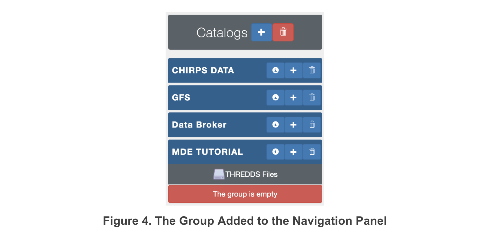
The dialog will close and the group will be added to the navigation panel (see Figure 4).
.
The dialog will close and the group will be added to the navigation panel (see Figure 4).
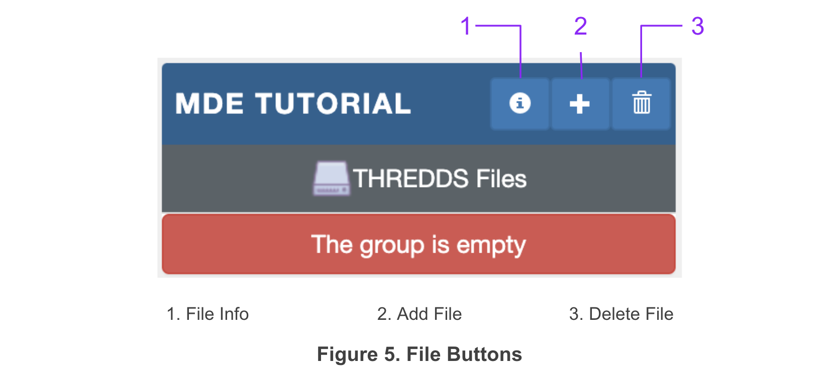
To add a file to a group, select the Add File Button located on the header of the created group (see Figure 5).
The Add a Thredds Server File dialog will appear (shown in Figure 6).
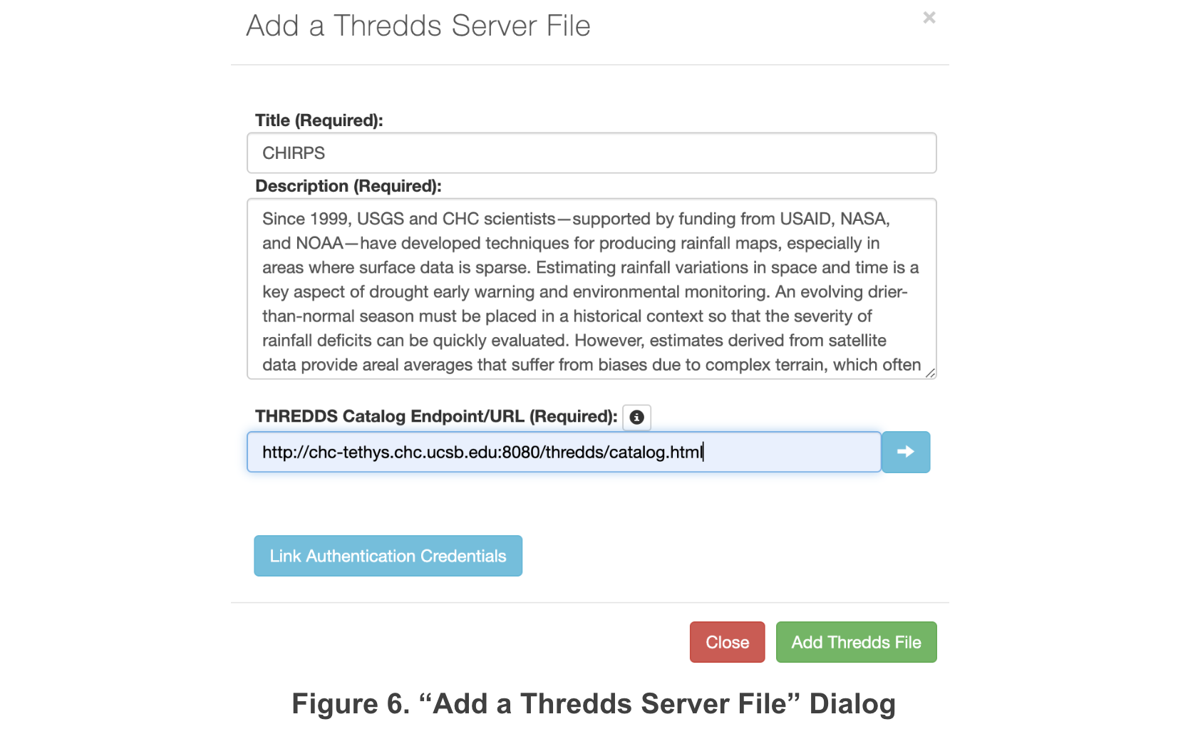
Enter a name and a description for the file. If the file requires user credentials (i.e. username and password) to
access, skip down and complete the section labeled Enter User Credentials for Files and then return and continue from
this point. Enter a URL for the THREDDS Catalog where the file is accessible. Click the Access Catalog Button  to
connect to the THREDDS Catalog.
to
connect to the THREDDS Catalog.
A separate dialog will appear listing the files and folders contained in the catalog at the specified URL (see Figure 7). Select a file or folder. If a folder is selected, the contents of the folder will be displayed in the dialog. If a file is selected, the variables, dimensions, and metadata for the file will be retrieved and loaded into the Add a Thredds Server File dialog (see Figure 8).


All the variables with two or more dimensions will be listed. Select the variables that you want included in the app and click the Add Thredds File button. The file will be added to the navigation panel under the group to which it was assigned (see Figure 9).

1.2.3. Enter User Credentials for File
Many datasets require a username and password to access the THREDDS Server. This feature was specifically added to the
app to allow access to data stored on the GES DISC data portal but it should be compatible with any server requiring
authentication. While the Add a Thredds Server File dialog is open, click the Link Authentication Credentials button  .
The Authentication dialog will appear (see Figure 10). If authentication has already been added to the app, click the
radio button next to the authentication you want to be associated with the app. To add authentication, fill in the
blanks in the Machine, User, and Password columns and press the add button
.
The Authentication dialog will appear (see Figure 10). If authentication has already been added to the app, click the
radio button next to the authentication you want to be associated with the app. To add authentication, fill in the
blanks in the Machine, User, and Password columns and press the add button  . Click the radio button next to the newly
added authentication and click save
. Click the radio button next to the newly
added authentication and click save  .
.

1.2.4. Data Discovery
To visualize the data on the map, select a file from the Navigation Panel (see Figure 11). The file will appear on the map and the Graph Window will open (see Figure 12).


The first variable listed in the file will be selected by default. The selected variable can be changed using the Variable dropdown. The dimensions associated with the variable will be listed along with the range of values spanned by each dimension. If the dimension is not a temporospatial dimension, the value associated with the dimension can be specified using the appropriate dropdown.
How the data is displayed on the map can be modified by changing the display settings located at the bottom of the
Graph Window. Set Data Bounds specifies the data values over which the color range on the map spans. The color style
can be specified using the Set Color Style dropdown. The opacity of the data on the map can be set using the Set Layer
Opacity slider. Once the display setting are set to your liking, click the Update Display Settings button  .
.

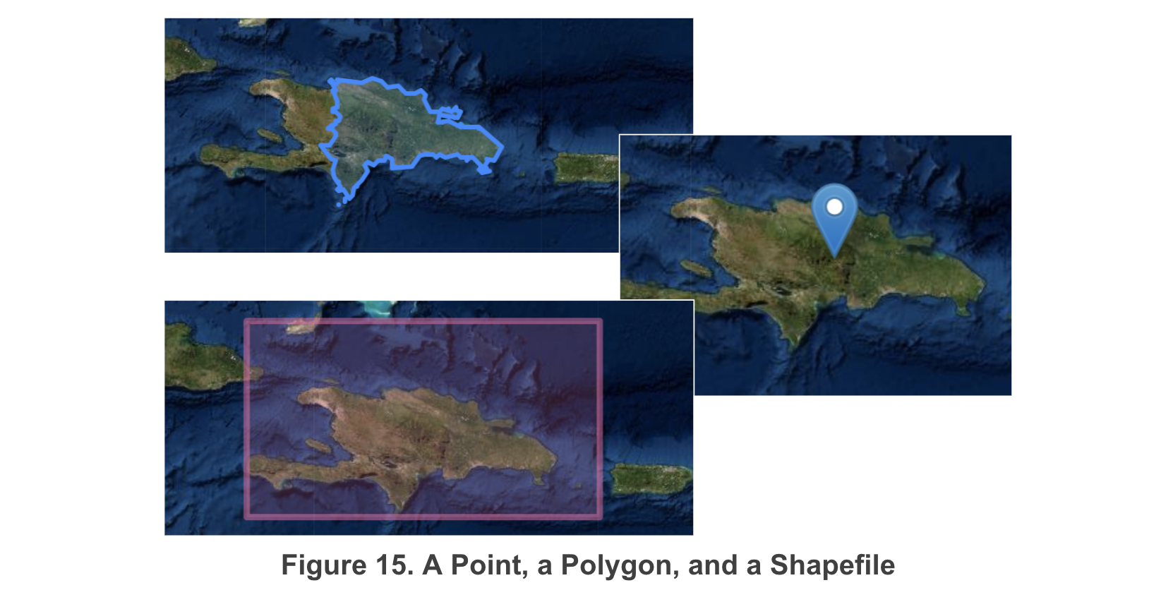
Data can be extracted at a point or over a user defined polygon. To extract the data at a point, create a point on
the map using the Create Marker  tool located on the drawing menu in the map window. The Create Rectangle
  or Create
Polygon
or Create
Polygon  tools can be used to define a polygon over which to extract the data. To use a shapefile to define a polygon,
change the Mask Data With
tools can be used to define a polygon over which to extract the data. To use a shapefile to define a polygon,
change the Mask Data With  dropdown to Use A Shapefile. The Select a Shapefile dialog will open (shown in Figure 14).
If the shapefile has previously been uploaded to the map, check the radio button next to the desired shapefile and
click the Use Shapefile button
dropdown to Use A Shapefile. The Select a Shapefile dialog will open (shown in Figure 14).
If the shapefile has previously been uploaded to the map, check the radio button next to the desired shapefile and
click the Use Shapefile button  .
.

To upload a new shapefile, click the Upload Shapefile button  . Follow the prompts to upload the file, click the radio
button next to the uploaded file, and click the Use Shapefile button.
. Follow the prompts to upload the file, click the radio
button next to the uploaded file, and click the Use Shapefile button.
Once a location over which to extract the data has been specified, click the Plot Time Series button  to extract and
graph the data. It may take several minutes to retrieve the data, depending on the current network speeds.
The time series will be plotted in the graph window (see Figure 16).
to extract and
graph the data. It may take several minutes to retrieve the data, depending on the current network speeds.
The time series will be plotted in the graph window (see Figure 16).

The time series can be downloaded as a csv or json file. Open the Download Data dropdown  and select the desired format.
An HTML file can also be downloaded which contains a web map that shows the same data that is displayed in the map
window. The last download option is to download a python notebook with code to extract the time series for the file
and variable currently selected in the MDE.
and select the desired format.
An HTML file can also be downloaded which contains a web map that shows the same data that is displayed in the map
window. The last download option is to download a python notebook with code to extract the time series for the file
and variable currently selected in the MDE.

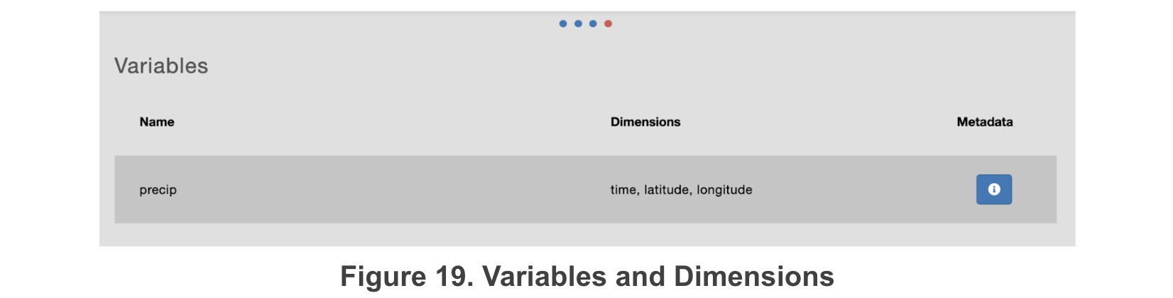
There are two more tabs in the graph window which can be examined by clicking the Move Right arrow ![]() located to the
right of the graph window. The first tab shows the metadata contained in the file (see Figure 18). The second tab
shows all the variables in the file with the associated dimensions (see Figure 19). The metadata for each variable
can be seen by clicking the Metadata Info button
located to the
right of the graph window. The first tab shows the metadata contained in the file (see Figure 18). The second tab
shows all the variables in the file with the associated dimensions (see Figure 19). The metadata for each variable
can be seen by clicking the Metadata Info button  . A dialog will open showing the variable metadata (see Figure 20).


1.3. Developers
MDE was originally developed by Enoch Jones and Elkin Giovanni Romero Bustamante at Brigham Young University’s (BYU) Hydroinformatics laboratory with the support of the World Meteorological Organization. The BYU’s Hydroinformatics laboratory focuses on delivering different software products and services for water modelling. Some of the most important works include: Global Streamflow Forecast Services API , creation of the Tethys Platform , and Hydroserver Lite . The most recent publications and works can be found on the BYU Hydroinformatics website.
1.4. Source Code
The MDE source code is available on Github: